How to use a spectrum analyser to find radiated emissions sources

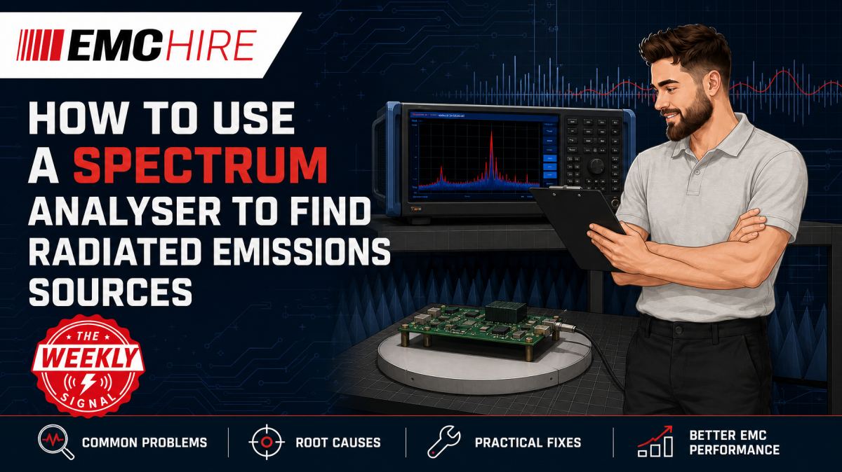
A spectrum analyser peak tells you where to look in frequency. It does not tell you whether the source is a clock edge, a switch-mode converter, a cable common-mode current or an enclosure resonance.

To find an emissions source efficiently, move through controlled stages: reproduce the peak, identify its frequency signature, determine the dominant coupling path, localise it with near-field probes, then confirm the diagnosis by making one reversible change.

Start with a repeatable radiated emissions pre-scan

Diagnosis becomes guesswork if the original peak cannot be reproduced. Before opening the enclosure or touching the PCB, record the equipment under test operating mode, software state, cable configuration, power source, peripherals, load condition, antenna polarisation and measurement geometry.

A spectrum analyser is useful for fast pre-scan and debugging work, but it is not automatically equivalent to a CISPR-compliant measuring receiver. Formal radiated emissions measurements may require specified detectors, bandwidths, antennas, distances, site characteristics and search procedures. The applicable product or product-family standard determines those details.

Radiated emissions measurements commonly start at 30 MHz, but neither the starting frequency nor the upper limit is universal. The required range may depend on the product standard, internal clock frequencies, radio functions and intended market. Check the latest active edition, product scope, limits, detector requirements and test configuration before treating a development scan as compliance evidence.

For initial investigation, capture a wide-span peak trace to identify candidate frequencies. Use analyser settings appropriate to the frequency range and applicable measurement method. A resolution bandwidth that is too wide can merge adjacent emissions and raise the displayed noise floor. One that is unnecessarily narrow slows the sweep and may hide intermittent behaviour if sweep time and event timing are poorly matched.

Peak detection is normally useful during exploratory scans because it responds quickly and is unlikely to under-report a narrow intermittent signal in the way an unsuitable averaging process might. Quasi-peak and average results have different meanings and must not be inferred from a peak trace. If comparison with a limit is required, use the detectors and bandwidths specified by the relevant standard.

Turn the peak frequency into a source hypothesis

Frequency correlation is the fastest first filter. Compare each suspect peak against oscillator frequencies, processor clocks, memory buses, display interfaces, switching regulators, motor drives and communication links. Do not inspect only the fundamental. Fast digital edges can produce harmonics far above the nominal clock frequency.

A 25 MHz clock, for example, may contribute energy at integer multiples extending well into the radiated measurement range. The strongest observed emission need not be at 25 MHz. PCB geometry, cable length, enclosure apertures and common-mode conversion can make a higher harmonic radiate more efficiently than the fundamental.

Look at peak spacing as well as absolute frequency. Evenly spaced lines often point towards a periodic clock or converter. Sidebands may indicate modulation by firmware activity, frame timing or load variation. A broad noise plateau is more consistent with fast switching edges, spread-spectrum clocking, unstable conversion or several unrelated sources than with one clean oscillator.

Use zero-span mode or a narrow span around the suspect frequency to examine timing. If the amplitude changes with display refresh, radio transmission, motor commutation or processor workload, that correlation is valuable. It is not proof. Two subsystems can share a power rail or timing event, so the apparent aggressor may only be modulating the actual source.

Manufacturer guidance should be checked for the specific analyser because sweep behaviour, preselector operation, detectors and overload indication vary. The Rohde & Schwarz spectrum analyser technical resources, for example, explain core analyser functions and measurement controls. Always use the operating manual for the actual model.

Rule out analyser overload and measurement artefacts

Spur hunting fails quickly when the analyser itself is generating the spurs. A strong nearby transmitter, EUT clock or probe signal can overload the input mixer and create intermodulation products that do not exist in the EUT emission.

Increase input attenuation and repeat the measurement. A genuine external signal should change predictably with the measurement path, while internally generated products may change disproportionately or disappear. Keep the preamplifier off until sensitivity is actually needed. Using high gain in the presence of strong signals reduces available dynamic range and can turn a clean spectrum into a forest of false responses.

Never connect an unknown conducted signal directly to the RF input. Confirm maximum input power, DC tolerance and required blocking or attenuation from the instrument documentation. Near-field probes can also produce unexpectedly high levels when placed directly over a high-current switching node.

Check the ambient spectrum with the EUT switched off, while keeping the rest of the arrangement unchanged. Broadcast services, mobile communications, laboratory computers and local switch-mode supplies can all resemble product emissions. An ambient line that coincides with the EUT frequency can still mask a genuine contribution, so compare amplitude, modulation and spatial behaviour rather than simply deleting it from the record.

Separate enclosure radiation from cable radiation

Many failed investigations focus on the PCB while ignoring the most efficient antenna in the setup: the attached cable. A signal is often generated differentially on the board, converted into common-mode current by impedance imbalance, then radiated by a power, data or peripheral cable.

Without disturbing the geometry more than necessary, use a suitable RF current probe around individual cables and observe the suspect frequency. The probe provides a relative conducted-current indication unless the complete measurement path is calibrated for quantitative current measurement. A strong correlation between cable current and the radiated peak points towards a common-mode path, but probe transfer impedance and analyser loading must be understood before assigning absolute dBµA values.

Move the cable slightly and watch the far-field or monitoring-antenna response. Large amplitude changes suggest that cable position and resonance are contributing. This is useful diagnostically, but the original standardised cable arrangement must be restored for comparable testing. Optimising cable placement until a peak disappears creates false confidence rather than a robust design.

A clamp ferrite can provide another reversible experiment. If fitting it to one cable suppresses both the cable current and radiated peak, investigate connector bonding, return-path discontinuities, filtering and common-mode conversion at that interface. The ferrite is evidence about the path, not necessarily the final production fix.

Localise PCB sources with near-field probes

Near-field probing is a localisation method, not a direct substitute for a calibrated far-field emissions test. Electric-field and magnetic-field probes respond differently, and their output depends strongly on probe orientation, spacing and construction.

A small magnetic loop is usually effective around high di/dt current loops, switch nodes, inductors, clock traces and return-path discontinuities. An electric-field probe is more responsive near high dv/dt conductors and poorly shielded nodes. Starting with a larger loop speeds area searching; changing to a smaller loop improves spatial discrimination at the cost of sensitivity.

Keep probe height and orientation consistent. Rotating a magnetic loop changes its coupling, while moving it a few millimetres can produce a large amplitude shift. If these variables are not controlled, a colourful hotspot map can reflect probe technique rather than source strength.

Use the analyser in a narrow span centred on the known emission, then scan methodically across functional blocks. Mark the locations producing the strongest response. The antennas and near-field probes available for EMC investigation should be selected according to frequency range, required spatial resolution and whether electric-field, magnetic-field or cable-current coupling is being investigated.

Do not assume the strongest local field is the dominant radiated source. A switch node can show a very high local amplitude yet couple poorly to the outside world. A weaker signal at a connector may drive a long cable and dominate the chamber result. Correlate the near-field indication with the original radiated peak.

Confirm causality with controlled changes

A diagnosis becomes credible when one reversible change produces the predicted response. Change only one variable at a time and retain before-and-after traces using identical analyser settings.

• Temporarily reduce or disable a suspect clock, where the product permits it safely.
• Change processor workload or interface activity without altering unrelated functions.
• Apply a small absorber, shield or conductive tape patch as a diagnostic experiment.
• Add a temporary common-mode ferrite to the suspected cable.
• Improve a connector bond using a short, low-inductance connection.
• Substitute a known power source or peripheral while preserving representative operation.

A long bonding lead is rarely a valid high-frequency experiment. Its inductance can prevent the intended RF bond from working, causing the engineer to reject a sound shielding hypothesis. Wide copper tape or a direct metal contact usually gives a more meaningful temporary bond.

Track amplitude trends rather than chasing a single displayed number. Probe position, analyser settings and EUT operating state all affect the result. Once a mitigation appears effective, repeat the radiated pre-scan in the original geometry. Local probe reduction alone does not establish that the far-field emission has improved.

Typical scenario

Consider an illustrative controller that produces a narrow radiated peak and several evenly spaced harmonics during a pre-scan. The team first records the exact operating mode and confirms that the lines disappear when the EUT is switched off. The spacing corresponds to a digital interface clock, but near-field probing finds similar frequencies around both the processor and an external cable connector.

A current probe around the cable shows a correlated response. Adding a temporary common-mode ferrite reduces the monitored radiated peak, while probing near the connector highlights a return-path discontinuity. The likely mechanism is not simply the clock trace radiating directly. Clock energy is being converted into common-mode cable current at the interface.

Changing the analyser, probe type or cable arrangement without a plan could lead the team towards the wrong PCB area. Early investigation instead directs attention to connector bonding, filter layout and reference-plane continuity before tooling or enclosure design is fixed.

EMC Hire can support this type of work with spectrum analysers, antennas, near-field probes, current probes and suitable accessories, alongside practical equipment-selection support. The EMC equipment selection guides provide a starting point, while the radiated emissions system information covers complete measurement arrangements. Where cable-borne noise may be feeding the radiated problem, the conducted emissions system information is also relevant.

When to Hire EMC Equipment

Hiring suits short debugging windows, irregular pre-compliance demand and project peaks where purchasing a complete measurement chain would leave equipment unused for much of its life. It also gives the team access to the correct frequency coverage, probes, antennas and accessories for the current programme rather than forcing an unsuitable instrument into service.

Ownership brings calibration planning, maintenance, storage, software and obsolescence costs. There is also a technical risk in buying around one immediate failure, only to discover that the next product requires different bandwidth, dynamic range or transducers. A defined hire period limits that exposure and avoids unnecessary capital expenditure.

EMC Hire uses test equipment with calibration traceable through an appropriate ISO/IEC 17025 accredited calibration provider where calibration is relevant to the measurement. Suitable traceable calibration supports repeatability, confidence in recorded data and better comparison between development and formal testing. It does not make an informal bench arrangement equivalent to a standardised compliance setup.

Teams can also use accessible pre-compliance testing to debug prototypes, gather calibrated engineering data and reduce late redesign risk before formal testing. EMC Hire can provide equipment hire, facility access, on-site testing and practical setup support, as well as formal compliance testing where appropriate for self-certification applications. The manufacturer remains responsible for identifying applicable legislation, standards, conformity assessment routes and technical file requirements.

Common EMC Testing Mistakes to Avoid

Changing cable geometry during every measurement

Cable movement changes antenna behaviour and common-mode impedance. If each mitigation is tested with a different cable position, amplitude changes cannot be attributed confidently to the design change.

Using near-field amplitude as a compliance result

A probe reading depends on probe geometry, orientation and distance. It can rank local sources under controlled conditions, but it does not directly predict a standardised field-strength result in dBµV/m.

Ignoring input overload

Excessive preamplifier gain or insufficient attenuation can generate analyser artefacts. Engineers may spend hours modifying circuitry to remove a spur that exists only inside the instrument.

Testing an unrepresentative operating mode

An idle processor, inactive display or unloaded converter may produce a clean scan that has little relevance to normal operation. Record worst-case or otherwise justified modes, including software, loads and peripheral activity.

Failing to preserve analyser settings

Changing resolution bandwidth, detector, attenuation or preamplifier state between traces invalidates direct amplitude comparisons. Save screenshots or trace files together with the complete instrument configuration.

Stopping after a local probe improvement

Reducing one PCB hotspot can shift current into another path. Repeat the original radiated pre-scan to establish whether the emission observed at the antenna has actually fallen.

Frequently Asked Questions (FAQs)

Can a spectrum analyser prove radiated emissions compliance?

Not by itself. Compliance depends on the complete measurement system, site, antenna factors, cable losses, detector behaviour, bandwidths, distance, EUT configuration and procedures required by the applicable product standard. A spectrum analyser can be highly effective for pre-scan and fault finding when used within its capabilities.

Should I use an electric-field or magnetic-field near-field probe?

Use a magnetic loop to investigate high-frequency current loops and high di/dt regions. An electric-field probe is useful around high dv/dt nodes and conductors. In practice, comparing both often reveals whether the dominant local coupling is magnetic or electric.

Why does the strongest harmonic move when the cable moves?

The cable is probably participating in the radiating structure. Its position changes coupling, common-mode impedance and resonance. Investigate the interface return path and common-mode current rather than treating cable routing as the permanent remedy.

How do I distinguish an ambient signal from an EUT emission?

Compare EUT-on and EUT-off traces, then examine timing, modulation and spatial response. Changing EUT operating mode can help. An ambient transmission may overlap an EUT emission, so disappearance is not always clean or complete.

What records should be kept during spur hunting?

Retain analyser settings, trace files, probe type and orientation, cable layout photographs, EUT software and operating mode, loads, peripherals, power arrangement and every temporary modification. Without that record, a later team may be unable to reproduce either the failure or the improvement.

Move from the peak to defensible evidence

A disciplined investigation links four things: the observed frequency, the circuit timing, the physical coupling path and the response to a controlled mitigation. That chain is far more useful than a collection of unexplained screenshots. It supports design decisions, formal test planning, technical documentation, EMC risk assessment and a more defensible compliance evidence trail.

For help selecting a spectrum analyser and probes, arranging equipment hire, booking space at the EMC Hire test facility, or discussing on-site, pre-compliance or formal compliance testing, contact the EMC Hire engineering team on +44 (0)1462 817111 or email sales@emchire.co.uk.